Video Link

影片连结

You can view the code used in this Episode here: SampleCode

您可以在此处查看 此剧 集中使用的代码： SampleCode

导入我们的数据 (Importing our Data)

The first step is to import our data into python.

第一步是将我们的数据导入python。

We can do that by going on the following link: Data

我们可以通过以下链接来做到这一点： 数据

Click on “code” and download ZIP.

单击“代码”并下载ZIP。

Locate WeatherDataP.csv and copy it into your local disc under a new file called ProjectData

找到WeatherDataP.csv并将其复制到本地磁盘下名为ProjectData的新文件下

Note: WeatherData.csv and WeahterDataM.csv were used in Simple Linear Regression and Multiple Linear Regression.

注意：WeatherData.csv和WeahterDataM.csv用于简单线性回归和多重线性回归 。

Now we are ready to import our data into our Notebook:

现在我们准备将数据导入到笔记本中：

How to set up a new Notebook can be found at the start of Episode 4.3

如何设置新笔记本可以在第4.3节开始时找到

Note: Keep this medium post on a split screen so you can read and implement the code yourself.

注意：请将此帖子张贴在分屏上，以便您自己阅读和实现代码。

# Import Pandas Library, used for data manipulation
# Import matplotlib, used to plot our data
# Import numpy for linear algebra operationsimport pandas as pd
import matplotlib.pyplot as plt
import numpy as np# Import our WeatherDataP.csv and store it in the variable rweather_data_pweather_data_p = pd.read_csv("D:\ProjectData\WeatherDataP.csv") 
# Display the data in the notebookweather_data_p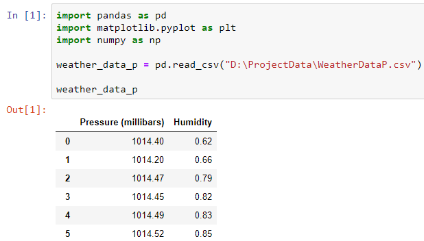

绘制数据 (Plotting our Data)

In order to check what kind of relationship Pressure forms with Humidity, we plot our two variables.

为了检查压力与湿度之间的关系，我们绘制了两个变量。

# Set our input x to Pressure, use [[]] to convert to 2D array suitable for model inputX = weather_data_p[["Pressure (millibars)"]]
y = weather_data_p.Humidity# Produce a scatter graph of Humidity against Pressureplt.scatter(X, y, c = "black")
plt.xlabel("Pressure (millibars)")
plt.ylabel("Humidity")

Here we see Humidity vs Pressure forms a bowl shaped relationship, reminding us of the function: y = 𝑥² .

在这里，我们看到湿度与压力之间呈碗形关系，使我们想起了函数y =𝑥²。

预处理我们的数据 (Preprocessing our Data)

This is the additional step we apply to polynomial regression, where we add the feature 𝑥² to our Model.

这是我们应用于多项式回归的附加步骤 ，在此步骤中将特征𝑥²添加到模型中。

# Import the function "PolynomialFeatures" from sklearn, to preprocess our data
# Import LinearRegression model from sklearnfrom sklearn.preprocessing import PolynomialFeatures
from sklearn.linear_model import LinearRegression# Set PolynomialFeatures to degree 2 and store in the variable pre_process
# Degree 2 preprocesses x to 1, x and x^2
# Degree 3 preprocesses x to 1, x, x^2 and x^3
# and so on..pre_process = PolynomialFeatures(degree=2)# Transform our x input to 1, x and x^2X_poly = pre_process.fit_transform(X)# Show the transformation on the notebookX_poly

e+.. refers to the position of the decimal place.

e + ..指小数位的位置。

E.g1.0e+00 = 1.0 [ keep the decimal point where it is ]1.0144e+03 = 1014.4 [ Move the decimal place 3 places to the right ]1.02900736e+06 = 1029007.36 [ Move the decimal place 6 to places to the right ]

例如 1.0e + 00 = 1.0 [保留小数点处的位置] 1.0144e + 03 = 1014.4 [将小数位右移3位] 1.02900736e + 06 = 1029007.36 [将小数点6向右移动]

— — — — — — — — — — — — — — — — — —

— — — — — — — — — — — — — — — — — — — —

The code above makes the following Conversion:

上面的代码进行了以下转换：

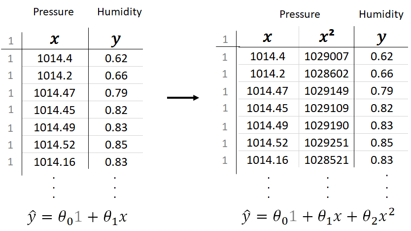
Notice that there is a hidden column of 1’s which can be thought of as the variable associated with θ₀. Since θ₀ × 1 = θ₀ this is often left out.

请注意，有一个隐藏的1列，可以将其视为与θ₀相关的变量。 由于θ₀×1 =θ₀，因此经常被忽略。

— — — — — — — — — — — — — — — — — —

— — — — — — — — — — — — — — — — — — — —

实现多项式回归 (Implementing Polynomial Regression)

The method here remains the same as multiple linear regression in python, but here we are fitting our regression model to the preprocessed data:

此处的方法与python中的多元线性回归相同，但此处我们将回归模型拟合为预处理的数据：

pr_model = LinearRegression()# Fit our preprocessed data to the polynomial regression modelpr_model.fit(X_poly, y)# Store our predicted Humidity values in the variable y_newy_pred = pr_model.predict(X_poly)# Plot our model on our dataplt.scatter(X, y, c = "black")
plt.xlabel("Pressure (millibars)")
plt.ylabel("Humidity")
plt.plot(X, y_pred)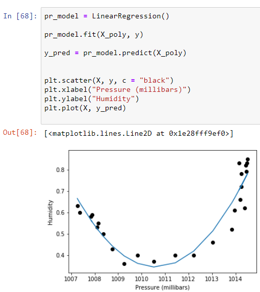

We can extract θ₀, θ₁ and θ₂ using the following code:

我们可以使用以下代码提取θ₀，θ₁和θ2 ：

theta0 = pr_model.intercept_
_, theta1, theta2 = pr_model.coef_theta0, theta1, theta2

A “_” is used to ignore the first value in pr_model.coef as this is given by default as 0. The other two co-efficients are labelled theta1 and theta 2 respectively.

“ _”用于忽略pr_model.coef中的第一个值，因为默认情况下该值为0。其他两个系数分别标记为theta1和theta 2。

Giving our polynomial regression model roughly as:

大致给出我们的多项式回归模型：

使用我们的回归模型进行预测 (Using our Regression Model to make predictions)

# Predict humidity for a pressure of 1007 millibars
# Tranform 1007 to 1, 1007, 1007^2 suitable for input, using 
# pre_process.fit_transformy_new = pr_model.predict(pre_process.fit_transform([[1007]]))
y_new

Here we expect a Humidity value of 0.7164631 for a pressure reading of 1007 millibars.

在这里，对于1007毫巴的压力读数，我们期望的湿度值为0.7164631。

We can plot this point on our data plot using the following code:

我们可以使用以下代码在数据图上绘制该点：

plt.scatter(1007, y_new, c = "red")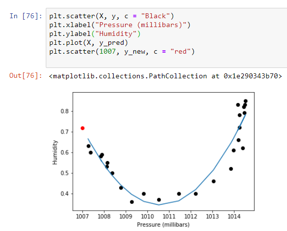

评估我们的模型 (Evaluating our Model)

To evaluate our model we are going to be using mean squared error (MSE), discussed in the previous episode, the function can easily be imported from sklearn.

为了评估我们的模型，我们将使用上一集中讨论的均方误差(MSE) ，可以轻松地从sklearn导入函数。

from sklearn.metrics import mean_squared_error
mean_squared_error(y, y_pred)

The mean squared error for our regression model is given by: 0.003358..

我们的回归模型的均方误差为：0.003358 ..

If we want to change our model to include 𝑥³ we can do so by simply changing PolynomialFeatures to degree 3:

如果要更改模型以包括𝑥³ ，可以通过将PolynomialFeatures更改为3级来实现 ：

pre_process = PolynomialFeatures(degree=3)

Let’s check if this has decreased our mean squared error:

让我们检查一下这是否降低了均方误差：

Indeed it has.

确实有。

You can change the degree used in PolynomialFeatures to anything you like and see for yourself what effect this has on our MSE.

您可以将PolynomialFeatures中使用的度数更改为您喜欢的任何值，并亲自查看这对我们的MSE有什么影响。

Ideally we want to choose the model that:

理想情况下，我们要选择以下模型：

• Has the lowest MSE

  MSE最低

• Does not over-fit our data

  不会过度拟合我们的数据

It is important that we plot our model on our data to ensure we don’t end up with the model shown at the end of Episode 4.6, which had an extremely low MSE but over-fitted our data.

重要的是， 我们需要在数据上绘制模型，以确保最终不会出现第4.6集末显示的模型，该模型的MSE极低，但数据过拟合。

上一集 - 下一集 (Prev Episode — Next Episode)

如有任何疑问，请留在下面！ (If you have any questions please leave them below!)