spotify歌曲下载

TL; DR (TL;DR)

Spotify is my favorite digital music service and I’m very passionate about the potential to extract meaningful insights from data. Therefore, I decided to do this article to consolidate my knowledge of some classification models and to contribute to the study of other beginners in Data Science.

Spotify是我最喜欢的数字音乐服务，我非常热衷于从数据中提取有意义的见解的潜力。因此，我决定写这篇文章来巩固我对一些分类模型的了解，并为研究数据科学的其他初学者做出贡献。

I constructed a dataset with 2755 hit and non-hit songs and extracted their audio features using the Spotipy library. I tested three classification models (Random Forest, Logistic Regression, and SVM) and choose the model with the best accuracy to predict what new songs would be hits.

我用2755首热门歌曲和未热门歌曲构建了一个数据集，并使用Spotipy库提取了它们的音频特征。我测试了三种分类模型(Random Forest，Logistic回归和SVM)，并选择了精度最高的模型来预测将要流行的新歌曲。

1.简介 (1. Introduction)

Spotify API provides full access to all music data available on Spotify. To access Spotify API, you have to register on the Spotify website dedicated to developers, select “Create an App”, register your information, and get your CLIENT_ID and CLIENT_SECRET. The API documentation and the data are easy to understand, maintained, and include essential metadata.

Spotify API提供对Spotify上所有可用音乐数据的完全访问权限。要访问Spotify API，您必须在专用于开发人员的Spotify网站上注册，选择“创建应用程序”，注册信息，并获取CLIENT_ID和CLIENT_SECRET。 API 文档和数据易于理解，维护，并包含必要的元数据。

We will try to discover what are the five artists that have more songs considered hits, what kind of music is most successful (positive or negative), and try to predict which songs in “Novidades da semana” can become a hit.

我们将尝试找出五首歌手中有更多歌曲被视为热门歌曲的艺术家，哪种音乐最成功(正或负)，并尝试预测“ Novidades da semana”中的哪些歌曲会成为热门歌曲。

2.数据集和功能 (2. Dataset and Features)

Using Spotipy library, I created two datasets:

使用Spotipy库，我创建了两个数据集：

2.1数据集 (2.1 dataset)

Composed of songs that are considered hits in the world, e.g., it was collected unique songs of the playlist “Top 50 by country” of all countries. These songs are considered as a hit (success = 1).The dataset is also composed of unique songs of random playlists from each genre (Sertanejo, Funk, Samba & Pagode, Rock, Jazz, Reggae, among others). These songs are considered as a non-hit (success = 0).That way, the dataset has 2755 songs considered hits and non-hits.

由世界上流行歌曲组成，例如，它是所有国家/地区的“国家排名前50位”播放列表中的独特歌曲。这些歌曲被视为热门歌曲(成功= 1)。数据集还由来自各流派(Sertanejo，Funk，Samba＆Pagode，Rock，Jazz，Reggae等)的随机播放列表的独特歌曲组成。这些歌曲被认为是非热门歌曲(成功= 0)。这样，数据集中有2755首歌曲被视为热门歌曲和非热门歌曲。

2.2测试仪 (2.2 test set)

The test set is composed of the best new releases “Novidades da semana” playlist that will be used to predict the probability of new songs become a hit.

测试集由最佳的新专辑“ Novidades da semana ”播放列表组成，这些播放列表将用于预测新歌流行的可能性。

More datails about how I created the datasets could be found at my Github repository.
在我的Github存储库中可以找到有关如何创建数据集的更多数据。

2.3特点 (2.3 Features)

Each track contains features categorized by track, artist and album information, and also audio analysis features. See more about the features HERE. The most relevant features for this article are explained in greater detail in later sections.

每个曲目都包含按曲目，艺术家和专辑信息分类的功能，以及音频分析功能。在此处查看有关功能的更多信息。与本文最相关的功能将在后面的部分中详细说明。

让我们开始吧！ (Let’s get started!)

3.导入库 (3. Import the libraries)

We will use pandas for data manipulation, NumPy for numerical computing, matplotlib and seaborn to data visualization, and sklearn for machine learning models, evaluation and dataset split.

我们将使用熊猫进行数据处理，使用NumPy进行数值计算，使用matplotlib和seaborn进行数据可视化，使用sklearn进行机器学习模型，评估和数据集拆分。

import pandas as pd
import numpy as np
import matplotlib.pyplot as plt
import seaborn as sns
from sklearn.preprocessing import MinMaxScaler
from sklearn.model_selection import train_test_split
from sklearn.ensemble import RandomForestClassifier
from sklearn.linear_model import LogisticRegression
from sklearn import svm
from sklearn.metrics import accuracy_score

The playlists “Top 50 by country” are updated daily and the “Novidades da semana” playlist, besides is updated every week, it could be different based on your profile. That way, the csv files contain the date that they were generated.

每天更新“国家排名前50”的播放列表，每周更新“ Novidades da semana”的播放列表，但根据您的个人资料，播放列表可能会有所不同。这样，csv文件将包含它们的生成日期。

dataset = pd.read_csv('spotifyAnalysis-08022020.csv')
test = pd.read_csv('predictSpotifyAnalysis-08022020.csv')

5.数据概述 (5. Data overview)

Let’s visualize the dataset and its features.

让我们可视化数据集及其特征。

dataset.head()

Using pandas.DataFrame.describe, we can see the following statistics and analyze the central tendency, dispersion and shape of a dataset’s distribution.

使用pandas.DataFrame.describe ，我们可以查看以下统计信息，并分析数据集分布的集中趋势，离散度和形状。

dataset.describe()

We can observe that tempo, key, duration_ms, loudness and popularity features are not on the same scale, so we will rescaling the data in the next section.

我们可以观察到速度，音调，duration_ms，响度和流行度功能不在同一个比例上，因此我们将在下一部分中重新缩放数据。

6.数据清理 (6. Data Cleaning)

There are no missing data and there is no need to treat categorical variables.

没有丢失的数据，也不需要处理分类变量。

6.1数据缩放 (6.1 Data Rescaling)

We will use the MinMaxScaler which rescaling is done independently between each column, in such a way that the new scale will be between 0 and 1 (or -1 and 1 if there are negative values in the dataset) and also preserves the original distribution.

我们将使用MinMaxScaler，它在每一列之间独立地进行重新缩放，这样新的缩放比例将在0和1之间(如果数据集中有负值，则在-1和1之间)并保留原始值分配。

MinMaxScaler subtracts each value by the lowest value in the column and then divides it by the difference between the maximum and minimum value.
MinMaxScaler用列中的最小值减去每个值，然后将其除以最大值和最小值之间的差。

# Rescaling tempo, key, duration_ms, loudness and popularity features.
scaler = MinMaxScaler()scaled_values = scaler.fit_transform(dataset[['tempo', 'key', 'duration_ms','loudness', 'popularity']]) 
dataset[['tempo', 'key', 'duration_ms','loudness', 'popularity']] = scaled_valuesscaled_values = scaler.fit_transform(test[['tempo', 'key', 'duration_ms','loudness', 'popularity']]) 
test[['tempo', 'key', 'duration_ms','loudness', 'popularity']] = scaled_values

7.探索性数据分析 (7. Exploratory Data Analysis)

7.1关联 (7.1 Correlation)

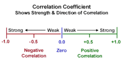
Correlation is a statistical technique to measure how variables are related.

关联是一种统计技术，用于衡量变量之间的关系。

Positive correlation: Indicates that the two variables move together.Negative correlation: Indicates that the two variables move in opposite directions.

正相关：表示两个变量一起移动。 负相关 ：指示两个变量沿相反方向移动。

plt.figure(figsize=(12,12))
corr = dataset.corr()
mask = np.zeros_like(corr, dtype=np.bool)
mask[np.triu_indices_from(mask, 1)] = True
sns.heatmap(corr, mask=mask, annot=True, cmap="Greens")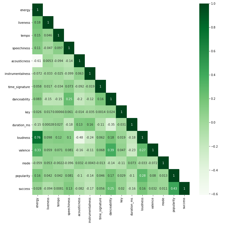

The variables with a stronger correlation are loudness x energy (strong and positive) and acousticness x energy (strong and negative).

相关性更强的变量是响度 x 能量 (强和正) 和声学 x 能量 (强和负)。

Loudness: The overall loudness of a track in decibels (dB). Loudness values are averaged across the entire track and are useful for comparing relative loudness of tracks. Loudness is the quality of a sound that is the primary psychological correlate of physical strength (amplitude). Values typical range between -60 and 0 db.
响度：轨道的整体响度，以分贝(dB)为单位。响度值是整个轨道的平均值，可用于比较轨道的相对响度。响度是声音的质量，它是身体力量(振幅)的主要心理关联。值的典型范围是-60至0 db。

Energy: Energy is a measure from 0.0 to 1.0 and represents a perceptual measure of intensity and activity. Typically, energetic tracks feel fast, loud, and noisy. For example, death metal has high energy, while a Bach prelude scores low on the scale. Perceptual features contributing to this attribute include dynamic range, perceived loudness, timbre, onset rate, and general entropy.
能量：能量是从0.0到1.0的量度，表示强度和活动的感知量度。通常，充满活力的曲目会感觉快速，响亮且嘈杂。例如，死亡金属具有较高的能量，而巴赫前奏的得分则较低。有助于此属性的感知特征包括动态范围，感知的响度，音色，发作率和一般熵。

Acousticness: A confidence measure from 0.0 to 1.0 of whether the track is acoustic. 1.0 represents high confidence the track is acoustic.
声学：轨道是否声学的置信度，范围为0.0到1.0。 1.0表示音轨是声学的高置信度。

Let’s visualize the correlation between the variables.

让我们可视化变量之间的相关性。

axis = ['ax0','ax1']
features = [['energy','loudness'],['energy','acousticness']]
colors = ['#48d66c', '#bd36d8']
titles = ['Energy x Loudness', 'Energy x Acousticness']
plot_dist_reg(1, 2, axis, features, colors, titles)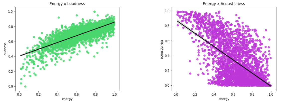

It can be concluded that tracks with higher energy tend to have higher volume in decibels (loudness) and tracks with less energy tend to be an acoustic song.

可以得出结论，具有较高能量的音轨往往具有较大的分贝(响度)音量，具有较低能量的音轨往往是声学歌曲。

7.2类的可视化 (7.2 Class visualization)

Let’s visualize the class distribution.

让我们可视化类分布。

plt.figure(1 , figsize = (15 , 5))
ax = sns.countplot(y = 'success', data = dataset, palette="Greens")
ax.set_title('Number of success (1) and non success (0) songs')
show_values_on_bars(ax, "h", 10)
plt.show()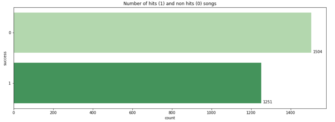

There are more non-hit songs then hit songs in the dataset.

数据集中的非流行歌曲比非流行歌曲多。

7.3热门歌曲 (7.3 Hit songs)

The next step is to analyze the songs considered as hits.

下一步是分析被视为热门歌曲。

# Get only hit songs
hits_df = dataset[dataset['success'] == 1]

What are the five artists that have more songs considered hit?

五位拥有更多歌曲的歌手被认为是热门？

top_artists = hits_df['artist'].value_counts()[:5]
name = top_artists.index.tolist()
amount = top_artists.values.tolist()plt.figure(1 , figsize = (15, 5))
ax = sns.barplot(x = name, y = amount, palette="Purples_d")
ax.set_title('Artists with more hit songs')
show_values_on_bars(ax, "v", 10)
plt.show()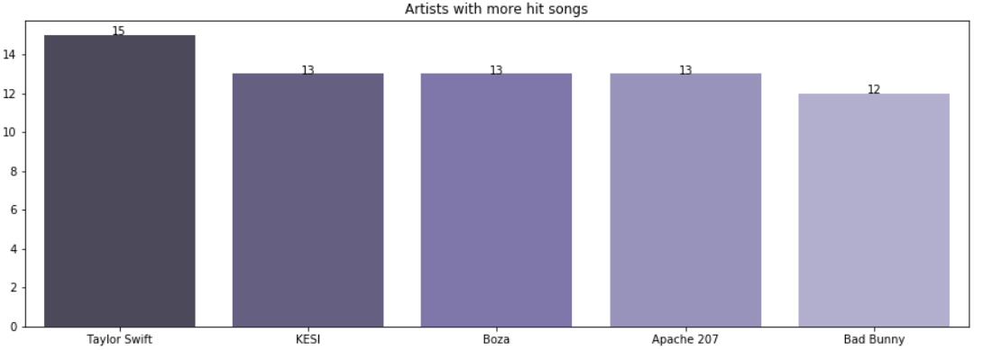

What kind of music is the most successful: positive or negative?

哪种音乐最成功：正面还是负面？

valence: A measure from 0.0 to 1.0 describing the musical positiveness conveyed by a track. Tracks with high valence sound more positive (e.g. happy, cheerful, euphoric), while tracks with low valence sound more negative (e.g. sad, depressed, angry).
价：从0.0到1.0的小节，描述了曲目传达的音乐积极性。价态高的音轨听起来更积极(例如，快乐，开朗，欣快)，而价态低的音轨听起来更加消极(例如，悲伤，沮丧，愤怒)。

To exemplify what is a song considered positive or negative, the song with the lowest valence (0.0349) in the dataset is Maia (Kamilo Sanclemente) and the song with the highest valence (0.9770) in the dataset is Corona (Minutemen).

为了举例说明什么是阳性或阴性歌曲，数据集中具有最低价(0.0349)的歌曲是Maia (Kamilo Sanclemente)，数据集中具有最高价(0.9770)的歌曲是Corona (Minutemen)。

valence = hits_df['valence'].value_counts()
valence_value = valence.index.tolist()
amount = valence.values.tolist()
i, high, low = 0, 0, 0for v in valence_value:
    if (float(v) >= 0.5):
        high += amount[i]
    else:
        low += amount[i]
    i += 1print('Positive tracks: ', high)
print('Negative tracks: ', low)output >>> Positive tracks: 704
           Negative tracks: 547

So, most hit songs are positive (happy, cheerful, euphoric).

因此，大多数热门歌曲都是正面的(快乐，开朗，欣快)。

8.机器学习建模与评估 (8. Machine Learning Modeling and Evaluation)

The dataset was split into training (70%) and test (30%).

数据集分为训练(70％)和测试(30％)。

# Split features and class data and drop irrelevant columns
X = dataset.drop(['success', 'artist', 'track_name'], axis=1).values
y = dataset[['success']].values# Split train and test set
X_train, X_test, y_train, y_test = train_test_split(X, y, test_size=0.3, random_state=0)

To predict whether a song will be a hit or not, we will use three different models (Random Forest, Logistic Regression and SVM) and select the best one based on the accuracy result.

为了预测歌曲是否会流行，我们将使用三种不同的模型(Random Forest，Logistic回归和SVM)，并根据准确性结果选择最佳的模型。

Accuracy is how close a measurement is to the true value.
精度是测量值与真实值的接近程度。

8.1随机森林 (8.1 Random Forest)

The random forest model combines a hundred of decision trees, each of which is trained on a different subset of the song features and different subset of the training data. The model makes a prediction, i.e., decides if a song is a hit or non-hit, performs a vote for each predicted result and then selects the prediction result with the most votes as the final prediction [3].

随机森林模型结合了一百个决策树，每个决策树都在歌曲特征的不同子集和训练数据的不同子集上进行训练。该模型进行预测，即确定歌曲是热门还是非热门，对每个预测结果进行投票，然后选择投票最多的预测结果作为最终预测[3]。

# Create the classifier object
rf_model = RandomForestClassifier(n_estimators = 100)# Train
rf_model.fit(X_train, y_train.ravel())# Predict
y_pred = rf_model.predict(X_test)print('Accuracy: ', accuracy_score(y_test, y_pred))output >>> Accuracy: 0.7315598548972189

8.2 Logistic回归 (8.2 Logistic Regression)

The logistic regression model linearly separates the data into two categories, i.e., predicts the probability of occurrence of a binary event utilizing a logit function and assigning a weight to each song feature, then uses these weights to predict whether a song is in the “hit” or “non-hit” category [4].

Logistic回归模型将数据线性地分为两类，即，使用logit函数预测二进制事件的发生概率，并为每首歌曲特征分配权重，然后使用这些权重来预测歌曲是否在“热门歌曲”中”或“非热门”类别[4]。

# Create the classifier object
lg_model = LogisticRegression()# Train
lg_model.fit(X_train, y_train.ravel())# Predict
y_pred = lg_model.predict(X_test)print('Accuracy: ', accuracy_score(y_test, y_pred))output >>> Accuracy: 0.6952841596130592

8.3支持向量机 (8.3 SVM)

The SVM model selects the best “hyperplane” (e.g., the “hyperplane” which has the maximum possible margin between support vectors) that separates the data into two categories [5].

SVM模型选择将数据分为两类的最佳“超平面”(例如，在支持向量之间具有最大可能余量的“超平面”)。

# Create the classifier object
svm_model = svm.SVC(kernel='linear')# Train
svm_model.fit(X_train, y_train.ravel())# Predict
y_pred = svm_model.predict(X_test)print('Accuracy: ', accuracy_score(y_test, y_pred))output >>> Accuracy: 0.6977025392986699

8.4评估 (8.4 Evaluation)

The accuracy of the 3 modeling methods are:

三种建模方法的准确性为：

Random Forest: 0.731Logistic Regression: 0.695SVM: 0.697

随机森林：0.731逻辑回归：0.695支持向量：0.697

9.结果 (9. Result)

As a result, the Random Forest model will be applied to predict the songs from “Novidades da semana” on Spotify.

结果，随机森林模型将用于预测Spotify上“ Novidades da semana”中的歌曲。

# Drop irrelevant columns
df_test = test.drop(['artist', 'track_name'], axis=1).values# Predict
test_predict = rf_model.predict(df_test)# Get only predict hit songs
hits_predict = (test_predict == 1).sum()
print(hits_predict, "out of", len(test_predict), "was predicted as HIT")output >>> 13 out of 60 was predicted as HIT

Which songs in “Novidades da semana” can become a hit? Let’s see the result.

“ Novidades da semana”中的哪些歌曲可以成为热门？让我们看看结果。

df = pd.DataFrame({'Song': test['track_name'], 'Artist': test['artist'], 'Predict': test_predict})
df.sort_values(by=['Predict'], inplace=True, ascending=False)
df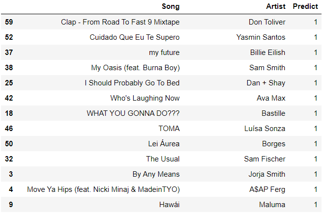

10.结论 (10. Conclusion)

Analyzing Spotify data on August 2nd, 2020, it could be concluded:

分析2020年8月2日的 Spotify数据，可以得出以下结论：

- The five artists who have more songs considered hits are Taylor Swift, KESI, Boza, Apache 207 and Bad Bunny.

-五位拥有更多热门歌曲的歌手是Taylor Swift，KESI，Boza，Apache 207和Bad Bunny 。

- Most hit songs are positive (happy, cheerful, euphoric).

-大多数热门歌曲都是正面的 (快乐，开朗，欣快)。

- The model with the best accuracy to predict what new songs will be hits is Random Forest.

-最准确地预测哪些新歌曲会流行的模型是Random Forest 。

- The songs of “Novidades da semana” that have a probability to be hits based on hits characteristics of “Top 50 by country” (all countries) are Clap From Road To Fast 9 Mixtape (Don Toliver), Cuidado Que Eu Te Supero (Yasmin Santos), my future (Billie Eilish), My Oasis feat. Burna Boy (Sam Smith), I Should Probably Go To Bed (Dan + Shay), Who’s Laughing Now (Ava Max), WHAT YOU GONNA DO??? (Bastille), TOMA (Luísa Sonza), Lei Áurea (Borges), The Usual (Sam Fischer), By Any Means (Jorja Smith), Move Ya Hips feat. Nicki Minaj & MadeinTYO (A$AP Ferg) and Hawái (Maluma).

-基于“按国家排名前50位”(所有国家/地区)的流行特征而很有可能被选为“ Novidades da semana”的歌曲，包括《 从公路到快9混音带》(Don Toliver)，《 Cuidado Que Eu Te Supero》( Yasmin Santos)，我的未来(Billie Eilish)，My Oasis壮举。 Burna Boy(Sam Smith)，我应该上床睡觉(Dan + Shay)，谁在笑(Ava Max)，您想做什么？？？ (巴士底狱)，托马(路易斯·桑萨)，雷阿雷亚(博格斯)，惯常(萨姆·菲舍尔)，通过任何方式(乔尔·史密斯)，莫亚·希普斯壮举。 Nicki Minaj和MadeinTYO(A $ AP Ferg)和Hawái(Maluma)。

请在此处查看完整的代码。 (See the complete code HERE.)

11.参考 (11. References)

[1] CORRELATIONAL ANALYSIS: POSITIVE, NEGATIVE AND ZERO CORRELATIONS. https://psychologyhub.co.uk/correlational-analysis-positive-negative-and-zero-correlations/
[1]相关分析：正，负和零相关。 https://psychologyhub.co.uk/correlational-analysis-positive-negative-and-zero-correlations/
[2] Song hit prediction: predicting billboard hits using Spotify data. arXiv:1908.08609 [cs.IR]. arxiv.org/abs/1908.08609
[2]歌曲匹配预测：使用Spotify数据预测广告牌匹配。 arXiv：1908.08609 [cs.IR]。 arxiv.org/abs/1908.08609
[3] NAVLANI, Avinash. Understanding Random Forests Classifiers in Python. https://www.datacamp.com/community/tutorials/random-forests-classifier-python
[3] NAVLANI，阿维纳什。了解Python中的随机森林分类器。 https://www.datacamp.com/community/tutorials/random-forests-classifier-python
[4] NAVLANI, Avinash. Understanding Logistic Regression in Python. https://www.datacamp.com/community/tutorials/understanding-logistic-regression-python
[4] NAVLANI，Avinash。了解Python中的逻辑回归。 https://www.datacamp.com/community/tutorials/understanding-logistic-regression-python
[5] NAVLANI, Avinash. Support Vector Machines with Scikit-learn. https://www.datacamp.com/community/tutorials/svm-classification-scikit-learn-python
[5] NAVLANI，阿维纳什。支持带有Scikit学习的矢量机。 https://www.datacamp.com/community/tutorials/svm-classification-scikit-learn-python