BikeDNA（五）参考数据的内在分析1

该笔记本分析用户提供的给定区域的参考自行车基础设施数据集的质量。 质量评估是“内在的”，即仅基于一个输入数据集，并且不使用数据集外部的信息。 对于将参考数据集与相应 OSM 数据进行比较的外在质量评估，请参阅笔记本 3a 和 3b。

该分析评估给定区域参考数据的“目的适应性”（Barron et al., 2014）。 分析的结果可能与自行车规划和研究相关 - 特别是对于包括自行车基础设施网络分析的项目，在这种情况下，几何拓扑尤为重要。

由于评估不使用外部参考数据集作为基本事实，因此无法对数据质量做出普遍的声明。 这个想法是让那些使用自行车网络的人能够评估他们的数据是否足以满足他们的特定用例。 该分析有助于发现潜在的数据质量问题，但将结果的最终解释权留给用户。

该笔记本利用了一系列先前调查 OSM/VGI 数据质量的项目的质量指标，例如 Ferster et al. (2020), Hochmair et al. (2015), Barron et al. (2014), and Neis et al. (2012).

此笔记本的输出文件（数据、地图、绘图）保存到 …/results/REFERENCE/[study_area]/ 子文件夹中。

# Load libraries, settings and dataimport json
import pickle
import warnings
from collections import Counter
import mathimport contextily as cx
import folium
import geopandas as gpd
import matplotlib as mpl
import matplotlib.pyplot as plt
import numpy as np
import osmnx as ox
import pandas as pd
import yaml
from matplotlib import cm, colorsfrom src import evaluation_functions as eval_func
from src import plotting_functions as plot_func%run ../settings/yaml_variables.py
%run ../settings/plotting.py
%run ../settings/tiledict.py
%run ../settings/load_refdata.py
%run ../settings/df_styler.py
%run ../settings/paths.pywarnings.filterwarnings("ignore")grid = ref_grid

D:\tmp_resource\BikeDNA-main\BikeDNA-main\scripts\settings\plotting.py:49: MatplotlibDeprecationWarning: The get_cmap function was deprecated in Matplotlib 3.7 and will be removed two minor releases later. Use ``matplotlib.colormaps[name]`` or ``matplotlib.colormaps.get_cmap(obj)`` instead.cmap = cm.get_cmap(cmap_name, n)
D:\tmp_resource\BikeDNA-main\BikeDNA-main\scripts\settings\plotting.py:46: MatplotlibDeprecationWarning: The get_cmap function was deprecated in Matplotlib 3.7 and will be removed two minor releases later. Use ``matplotlib.colormaps[name]`` or ``matplotlib.colormaps.get_cmap(obj)`` instead.cmap = cm.get_cmap(cmap_name)Reference graphs loaded successfully!
Reference data loaded successfully!<string>:49: MatplotlibDeprecationWarning: The get_cmap function was deprecated in Matplotlib 3.7 and will be removed two minor releases later. Use ``matplotlib.colormaps[name]`` or ``matplotlib.colormaps.get_cmap(obj)`` instead.
<string>:46: MatplotlibDeprecationWarning: The get_cmap function was deprecated in Matplotlib 3.7 and will be removed two minor releases later. Use ``matplotlib.colormaps[name]`` or ``matplotlib.colormaps.get_cmap(obj)`` instead.

1.数据完整性

1.1 网络密度

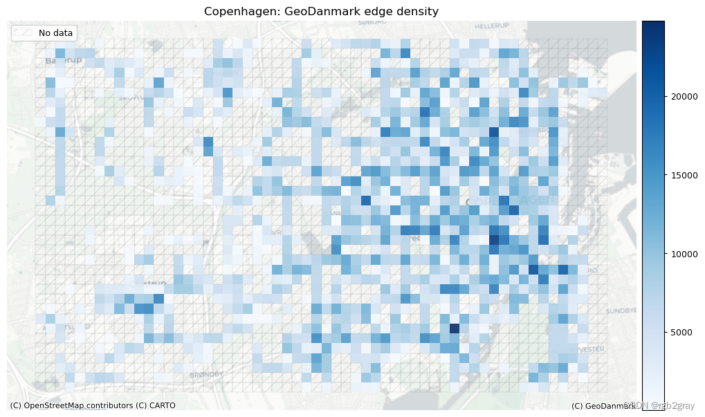
在此设置中，网络密度是指边的长度或每平方公里的节点数。 这是空间（道路）网络中网络密度的通常定义，它与网络科学中更常见的“结构”网络密度不同。 如果不与参考数据集进行比较，网络密度本身并不表明空间数据质量。 然而，对于熟悉研究区域的任何人来说，网络密度可以表明该区域的某些部分是否映射不足或过度。

方法

这里的密度不是基于边缘的几何长度，而是基于基础设施的计算长度。 例如，一条 100 米长的双向路径贡献了 200 米的自行车基础设施。 该方法用于考虑绘制自行车基础设施的不同方式，否则可能会导致网络密度出现较大偏差。 使用“compute_network_densis”，可以计算每单位面积的元素数量（节点、悬空节点和基础设施总长度）。 密度计算两次：首先计算整个网络的研究区域（“全局密度”），然后计算每个网格单元（“局部密度”）。 全局和局部密度都是针对整个网络以及受保护和未受保护的基础设施计算的。

解释

由于此处进行的分析是内在的，即不使用外部信息，因此无法知道低密度值是由于测绘不完整还是由于该地区实际缺乏基础设施所致。 然而，网格单元密度值的比较可以提供一些见解，例如：

• 基础设施密度低于平均水平表明局部网络较为稀疏
• 高于平均节点密度表明网格单元内交叉点相对较多
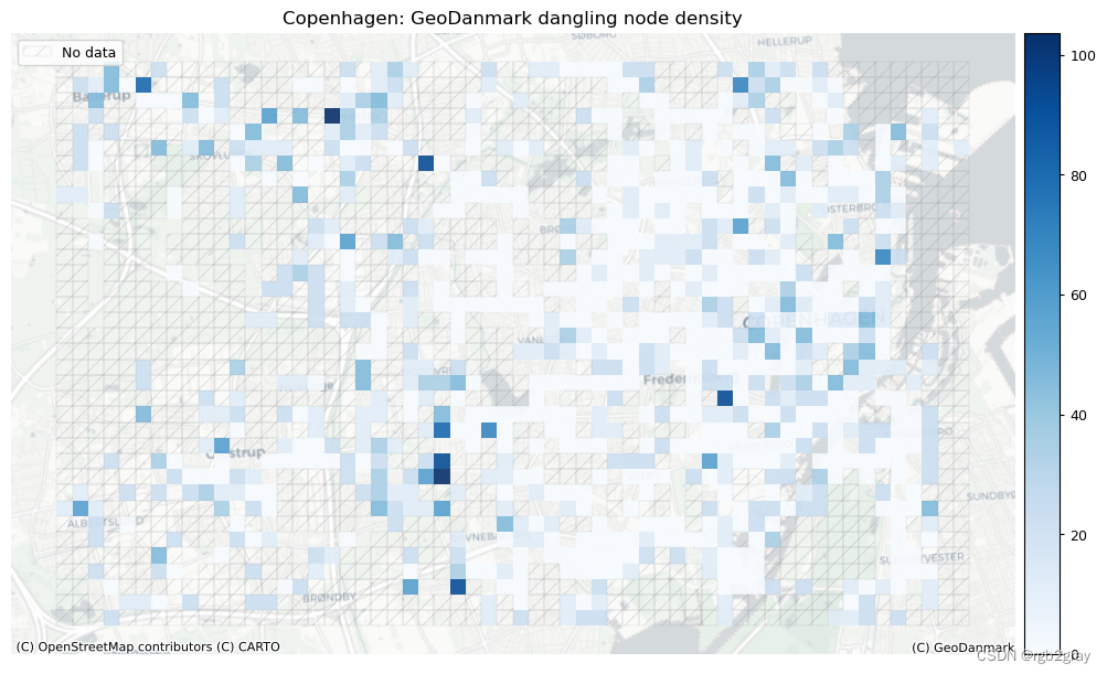
• 悬挂节点密度高于平均水平表明网格单元中存在相对较多的死角

全球网络密度

# Entire study area
edge_density, node_density, dangling_node_density = eval_func.compute_network_density((ref_edges_simplified, ref_nodes_simplified),grid.unary_union.area,return_dangling_nodes=True,
)density_results = {}
density_results["edge_density_m_sqkm"] = edge_density
density_results["node_density_count_sqkm"] = node_density
density_results["dangling_node_density_count_sqkm"] = dangling_node_densityref_protected = ref_edges_simplified.loc[ref_edges_simplified.protected == "protected"]
ref_unprotected = ref_edges_simplified.loc[ref_edges_simplified.protected == "unprotected"
]
ref_mixed = ref_edges_simplified.loc[ref_edges_simplified.protected == "mixed"]ref_data = [ref_protected, ref_unprotected, ref_mixed]
labels = ["protected_density", "unprotected_density", "mixed_density"]for data, label in zip(ref_data, labels):if len(data) > 0:ref_edge_density_type, _ = eval_func.compute_network_density((data, ref_nodes_simplified),grid.unary_union.area,return_dangling_nodes=False,)density_results[label + "_m_sqkm"] = ref_edge_density_typeelse:density_results[label + "_m_sqkm"] = 0protected_edge_density = density_results["protected_density_m_sqkm"]
unprotected_edge_density = density_results["unprotected_density_m_sqkm"]
mixed_protection_edge_density = density_results["mixed_density_m_sqkm"]print(f"For the entire study area, there are:")
print(f"- {edge_density:.2f} meters of bicycle infrastructure per km2.")
print(f"- {node_density:.2f} nodes in the bicycle network per km2.")
print(f"- {dangling_node_density:.2f} dangling nodes in the bicycle network per km2."
)
print(f"- {protected_edge_density:.2f} meters of protected bicycle infrastructure per km2."
)
print(f"- {unprotected_edge_density:.2f} meters of unprotected bicycle infrastructure per km2."
)
print(f"- {mixed_protection_edge_density:.2f} meters of mixed protection bicycle infrastructure per km2."
)

For the entire study area, there are:
- 3453.85 meters of bicycle infrastructure per km2.
- 22.74 nodes in the bicycle network per km2.
- 4.80 dangling nodes in the bicycle network per km2.
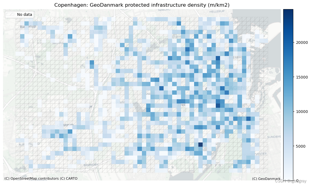
- 2998.80 meters of protected bicycle infrastructure per km2.
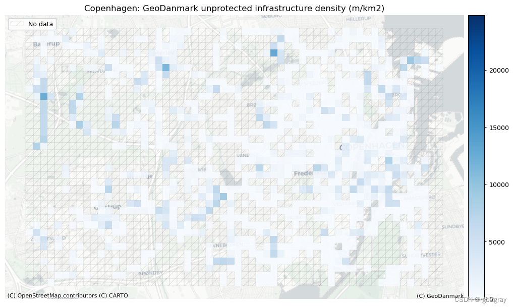
- 455.05 meters of unprotected bicycle infrastructure per km2.
- 0.00 meters of mixed protection bicycle infrastructure per km2.

# Save stats to csv
pd.DataFrame({"metric": ["meters of bicycle infrastructure per square km","nodes in the bicycle network per square km","dangling nodes in the bicycle network per square km","meters of protected bicycle infrastructure per square km","meters of unprotected bicycle infrastructure per square km","meters of mixed protection bicycle infrastructure per square km",],"value": [np.round(edge_density, 2),np.round(node_density, 2),np.round(dangling_node_density, 2),np.round(protected_edge_density, 2),np.round(unprotected_edge_density, 2),np.round(mixed_protection_edge_density, 2),],}
).to_csv(ref_results_data_fp + "stats_area.csv", index=False)

本地网络密度

# Per grid cell
results_dict = {}
data = (ref_edges_simp_joined, ref_nodes_simp_joined.set_index("osmid"))[eval_func.run_grid_analysis(grid_id,data,results_dict,eval_func.compute_network_density,grid["geometry"].loc[grid.grid_id == grid_id].area.values[0],return_dangling_nodes=True,)for grid_id in grid_ids
]results_df = pd.DataFrame.from_dict(results_dict, orient="index")
results_df.reset_index(inplace=True)
results_df.rename(columns={"index": "grid_id",0: "ref_edge_density",1: "ref_node_density",2: "ref_dangling_node_density",},inplace=True,
)grid = eval_func.merge_results(grid, results_df, "left")ref_protected = ref_edges_simp_joined.loc[ref_edges_simp_joined.protected == "protected"
]
ref_unprotected = ref_edges_simp_joined.loc[ref_edges_simp_joined.protected == "unprotected"
]
ref_mixed = ref_edges_simp_joined.loc[ref_edges_simp_joined.protected == "mixed"]ref_data = [ref_protected, ref_unprotected, ref_mixed]ref_labels = ["ref_protected_density", "ref_unprotected_density", "ref_mixed_density"]for data, label in zip(ref_data, ref_labels):if len(data) > 0:results_dict = {}data = (ref_edges_simp_joined.loc[data.index], ref_nodes_simp_joined)[eval_func.run_grid_analysis(grid_id,data,results_dict,eval_func.compute_network_density,grid["geometry"].loc[grid.grid_id == grid_id].area.values[0],)for grid_id in grid_ids]results_df = pd.DataFrame.from_dict(results_dict, orient="index")results_df.reset_index(inplace=True)results_df.rename(columns={"index": "grid_id", 0: label}, inplace=True)results_df.drop(1, axis=1, inplace=True)grid = eval_func.merge_results(grid, results_df, "left")

# Network density grid plotsset_renderer(renderer_map)
plot_cols = ["ref_edge_density", "ref_node_density", "ref_dangling_node_density"]
plot_titles = [area_name + f": {reference_name} edge density",area_name + f": {reference_name} node density",area_name + f": {reference_name} dangling node density",
]
filepaths = [ref_results_static_maps_fp + "density_edge_reference",ref_results_static_maps_fp + "density_node_reference",ref_results_static_maps_fp + "density_danglingnode_reference",
]
cmaps = [pdict["pos"], pdict["pos"], pdict["pos"]]
no_data_cols = ["count_ref_edges", "count_ref_nodes", "count_ref_nodes"]plot_func.plot_grid_results(grid=grid,plot_cols=plot_cols,plot_titles=plot_titles,filepaths=filepaths,cmaps=cmaps,alpha=pdict["alpha_grid"],cx_tile=cx_tile_2,no_data_cols=no_data_cols,attr=reference_name
)

受保护和未受保护基础设施的密度

在 BikeDNA 中，“受保护的基础设施”是指通过高架路缘、护柱或其他物理屏障等与汽车交通分开的所有自行车基础设施，或者不毗邻街道的自行车道。

不受保护的基础设施是专门供骑自行车者使用的所有其他类型的车道，但仅通过汽车交通分隔，例如街道上的画线。

# Network density grid plotsset_renderer(renderer_map)
plot_cols = ["ref_protected_density", "ref_unprotected_density", "ref_mixed_density"]plot_cols = [p for p in plot_cols if p in grid.columns]plot_titles = [area_name + f": {reference_name} protected infrastructure density (m/km2)",area_name + f": {reference_name} unprotected infrastructure density (m/km2)",area_name + f": {reference_name} mixed protection infrastructure density (m/km2)"
]# plot_titles = plot_titles[0:len(plot_cols)]filepaths = [ref_results_static_maps_fp + "density_protected_reference",ref_results_static_maps_fp + "density_unprotected_reference",ref_results_static_maps_fp + "density_mixed_reference",
]cmaps = [pdict["pos"]] * len(plot_cols)
no_data_cols = ["ref_protected_density", "ref_unprotected_density", "ref_mixed_density"]
norm_min = [0] * len(plot_cols)
norm_max = [max(grid[plot_cols].fillna(value=0).max())] * len(plot_cols)plot_func.plot_grid_results(grid=grid,plot_cols=plot_cols,plot_titles=plot_titles,filepaths=filepaths,cmaps=cmaps,alpha=pdict["alpha_grid"],cx_tile=cx_tile_2,no_data_cols=no_data_cols,use_norm=True,norm_min=norm_min,norm_max=norm_max,attr=reference_name
)

2.网络拓扑结构

本节探讨数据的几何和拓扑特征。 例如，这些是网络密度、断开的组件和悬空（一级）节点。 它还包括探索是否存在彼此非常接近但不共享边缘的节点（边缘下冲的潜在迹象），或者是否存在相交边缘而在相交处没有节点，这可能表明存在数字化错误，该错误将导致数字化错误。 扭曲网络上的路由。

由于大多数自行车网络的分散性，许多指标（例如缺失链接或网络间隙）可以简单地反映基础设施的真实范围(Natera Orozco et al., 2020)。 这对于道路网络来说是不同的，例如，断开的组件更容易被解释为数据质量问题。 因此，分析仅将非常小的网络间隙视为潜在的数据质量问题。

2.1 简化结果

为了比较网络中节点和边之间的结构和真实比率，通过删除所有间隙节点，在笔记本“1b”中创建了仅包括端点和交叉点处的节点的简化网络表示。

比较简化前后网络的度分布是对简化例程的快速健全性检查。 通常，非简化网络中的绝大多数节点都是二级节点； 然而，在简化的网络中，大多数节点的度数不是二。 仅在两种情况下保留二级节点：如果它们代表两种不同类型的基础设施之间的连接点； 或者如果需要它们以避免自循环（起点和终点相同的边）或同一对节点之间的多个边。

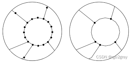
非简化网络（左）和简化网络（右）。

方法

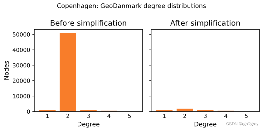
简化前后的节点度分布如下图所示。

解释

通常，节点度分布将从高（简化前）到低（简化后）二度节点计数，而对于所有其他度（1 或 3 及更高），它不会改变。 此外，节点总数将出现大幅下降。 如果简化后的图仍然保持相对较高的二度节点数量，或者简化后具有其他度数的节点数量发生变化，则这可能表明图转换或简化过程存在问题。

# Decrease in network elements after simplificationedge_percent_diff = (len(ref_edges) - len(ref_edges_simplified)) / len(ref_edges) * 100
node_percent_diff = (len(ref_nodes) - len(ref_nodes_simplified)) / len(ref_nodes) * 100simplification_results = {"edge_percent_diff": edge_percent_diff,"node_percent_diff": node_percent_diff,
}print(f"Simplifying the network decreased the number of edges with {edge_percent_diff:.1f}% and the number of nodes with {node_percent_diff:.1f}%."
)

Simplifying the network decreased the number of edges with 91.2% and the number of nodes with 92.2%.

# Node degree distributionset_renderer(renderer_plot)
fig, ax = plt.subplots(1, 2, figsize=pdict["fsbar_short"], sharey=True)degree_sequence_before = sorted((d for n, d in ref_graph.degree()), reverse=True)
degree_sequence_after = sorted((d for n, d in ref_graph_simplified.degree()), reverse=True
)ax[0].bar(*np.unique(degree_sequence_before, return_counts=True), tick_label = np.unique(degree_sequence_before), color=pdict["ref_base"])
ax[0].set_title("Before simplification")
ax[0].set_xlabel("Degree")
ax[0].set_ylabel("Nodes")ax[1].bar(*np.unique(degree_sequence_after, return_counts=True), tick_label = np.unique(degree_sequence_after), color=pdict["ref_base"])
ax[1].set_title("After simplification")
ax[1].set_xlabel("Degree")plt.suptitle(f"{area_name}: {reference_name} degree distributions")fig.tight_layout()plot_func.save_fig(fig, ref_results_plots_fp + "degree_dist_reference")
plt.show();

2.2 悬空节点

悬空节点是一阶节点，即它们仅附有一条边。 大多数网络自然会包含许多悬空节点。 悬空节点可能出现在实际的死胡同（代表死胡同）或某些特征的端点处，例如 当自行车道在街道中间结束时。 但是，在出现过冲/下冲的情况下，悬空节点也可能会作为数据质量问题出现（请参阅下一节）。 网络中悬空节点的数量在某种程度上也取决于数字化方法，如下图所示。

因此，悬空节点的存在本身并不是数据质量低的标志。 然而，在未知包含许多死胡同的区域中存在大量悬空节点可能表明数字化错误和边缘上冲/下冲问题。

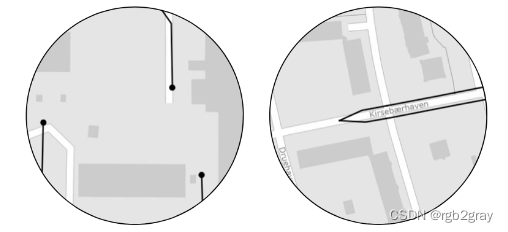
左：悬挂节点出现在道路要素结束处。 右：但是，当最后连接单独的特征时，将不会有悬空节点。

方法

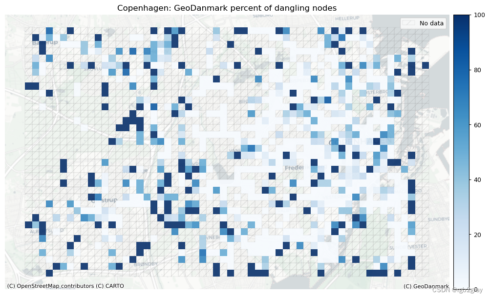
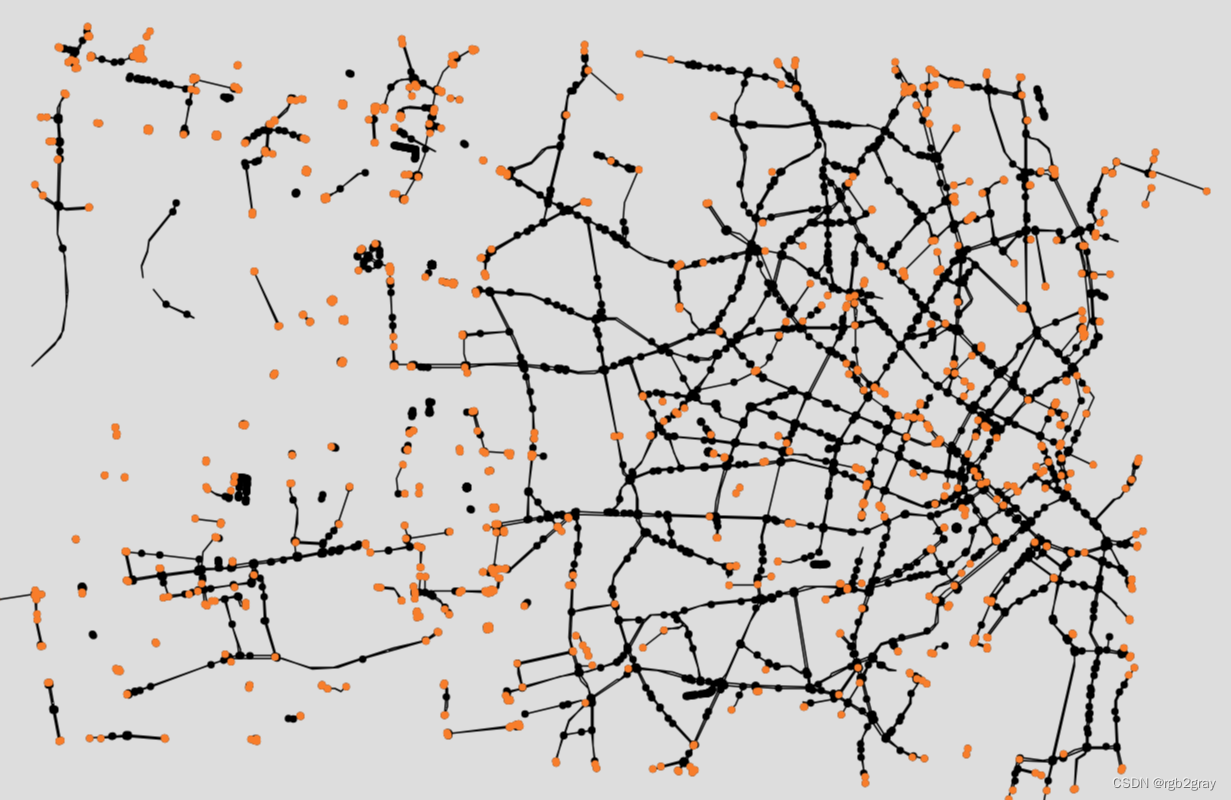
下面，在“get_dangling_nodes”的帮助下获得了所有悬空节点的列表。 然后，绘制包含所有节点的网络。 悬空节点以颜色显示，所有其他节点以黑色显示。

解释

我们建议进行可视化分析，以解释悬挂节点的空间分布，特别注意悬挂节点密度高的区域。 重要的是要了解悬挂节点的来源：它们是真正的死胡同还是数字化错误（例如，过冲/下冲）？ 数字化错误数量越多表明数据质量越低。

# Compute number of dangling nodes
dangling_nodes = eval_func.get_dangling_nodes(ref_edges_simplified, ref_nodes_simplified
)# Export results
dangling_nodes.to_file(ref_results_data_fp + "dangling_nodes.gpkg", index=False)# Compute local count and pct of dangling nodes
dn_ref_joined = gpd.overlay(dangling_nodes, grid[["geometry", "grid_id"]], how="intersection"
)
df = eval_func.count_features_in_grid(dn_ref_joined, "ref_dangling_nodes")
grid = eval_func.merge_results(grid, df, "left")grid["ref_dangling_nodes_pct"] = np.round(100 * grid.count_ref_dangling_nodes / grid.count_ref_simplified_nodes, 2
)# set to zero where there are simplified nodes but no dangling nodes
grid["ref_dangling_nodes_pct"].loc[grid.count_ref_simplified_nodes.notnull() & grid.ref_dangling_nodes_pct.isnull()
] = 0

# Plot dangling nodesset_renderer(renderer_map)
fig, ax = plt.subplots(1, figsize=pdict["fsmap"])from mpl_toolkits.axes_grid1 import make_axes_locatable
divider = make_axes_locatable(ax)
cax = divider.append_axes("right", size="3.5%", pad="1%")grid.plot(cax=cax,column="ref_dangling_nodes_pct",ax=ax,alpha=pdict["alpha_grid"],cmap=pdict["pos"],legend=True,
)# add no data patches
grid[grid["count_ref_simplified_nodes"].isnull()].plot(cax=cax,ax=ax,facecolor=pdict["nodata_face"],edgecolor=pdict["nodata_edge"],linewidth= pdict["line_nodata"],hatch=pdict["nodata_hatch"],alpha= pdict["alpha_nodata"],
)ax.legend(handles=[nodata_patch], loc="upper right")
ax.set_title(f"{area_name}: {reference_name} percent of dangling nodes")
ax.set_axis_off()
cx.add_basemap(ax=ax, crs=study_crs, source=cx_tile_2)
cx.add_attribution(ax=ax, text=f"(C) {reference_name}")
txt = ax.texts[-1]
txt.set_position([1,0.00])
txt.set_ha('right')
txt.set_va('bottom')plot_func.save_fig(fig,ref_results_static_maps_fp + "pct_dangling_nodes_reference")

# Interactive plot of dangling nodesedges_simplified_folium = plot_func.make_edgefeaturegroup(gdf=ref_edges_simplified,mycolor=pdict["base"],myweight=pdict["line_base"],nametag="Edges",show_edges=True,
)nodes_simplified_folium = plot_func.make_nodefeaturegroup(gdf=ref_nodes_simplified,mysize=pdict["mark_base"],mycolor=pdict["base"],nametag="All nodes",show_nodes=True,
)dangling_nodes_folium = plot_func.make_nodefeaturegroup(gdf=dangling_nodes,mysize=pdict["mark_emp"],mycolor=pdict["ref_base"],nametag="Dangling nodes",show_nodes=True,
)m = plot_func.make_foliumplot(feature_groups=[edges_simplified_folium,nodes_simplified_folium,dangling_nodes_folium,],layers_dict=folium_layers,center_gdf=ref_nodes_simplified,center_crs=ref_nodes_simplified.crs,attr=reference_name
)bounds = plot_func.compute_folium_bounds(ref_nodes_simplified)
m.fit_bounds(bounds)m.save(ref_results_inter_maps_fp + "folium_danglingmap_reference.html")display(m)

print("Interactive map saved at " + ref_results_inter_maps_fp.lstrip("../") + "folium_danglingmap_reference.html")

Interactive map saved at results/REFERENCE/cph_geodk/maps_interactive/folium_danglingmap_reference.html

2.3 下冲/过冲

当简化网络中的两个节点放置在几米距离内但不共享公共边缘时，通常是由于边缘上冲/下冲或其他数字化错误造成的。 当两个特征应该相交，但实际上彼此非常接近时，就会发生下冲。 当两个特征相遇并且其中一个特征超出另一个特征时，就会发生超调。 请参见下图的说明。 有关过冲/下冲的更详细说明，请参阅 GIS Lounge 网站。

左：当两条线要素未正确连接时（例如在交叉点处），会发生下冲。 右图：过冲是指线要素在相交线处延伸太远，而不是在相交处结束的情况。

方法

*下冲：*首先，“length_tolerance”（以米为单位）在下面的单元格中定义。 然后，使用“find_undershoots”，所有之间距离最大为“length_tolerance”的悬空节点对都被识别为下冲，并绘制结果。

*超调：*首先，“长度公差”（以米为单位）在下面的单元格中定义。 然后，使用“find_overshoots”，所有附加有悬空节点且最大长度为“length_tolerance”的网络边都被识别为过冲，并绘制结果。

过冲/下冲检测方法的灵感来自于 Neis et al. (2012)。

解释

欠调/过调不一定总是数据质量问题 - 它们可能是网络状况或数字化策略的准确表示。 例如，自行车道可能在转弯后不久突然结束，从而导致超调。 受保护的自行车道有时会被数字化为在交叉路口中断，从而导致交叉路口下冲。

过冲/下冲对数据质量影响的解释取决于上下文。 对于某些应用，例如路由，过冲并不构成特殊的挑战； 然而，鉴于它们扭曲了网络结构，它们可能会给网络分析等其他应用带来问题。 相反，下冲对于路线应用来说是一个严重的问题，特别是如果只考虑自行车基础设施的话。 它们还给网络分析带来了问题，例如对于任何基于路径的度量，例如大多数中心性度量，如介数中心性。

# USER INPUT: LENGTH TOLERANCE FOR OVER- AND UNDERSHOOTS
length_tolerance_over = 3
length_tolerance_under = 3for s in [length_tolerance_over, length_tolerance_under]:assert isinstance(s, int) or isinstance(s, float), print("Settings must be integer or float values!")print(f"Running overshoot analysis with a tolerance threshold of {length_tolerance_over} m.")
print(f"Running undershoot analysis with a tolerance threshold of {length_tolerance_under} m.")

Running overshoot analysis with a tolerance threshold of 3 m.
Running undershoot analysis with a tolerance threshold of 3 m.

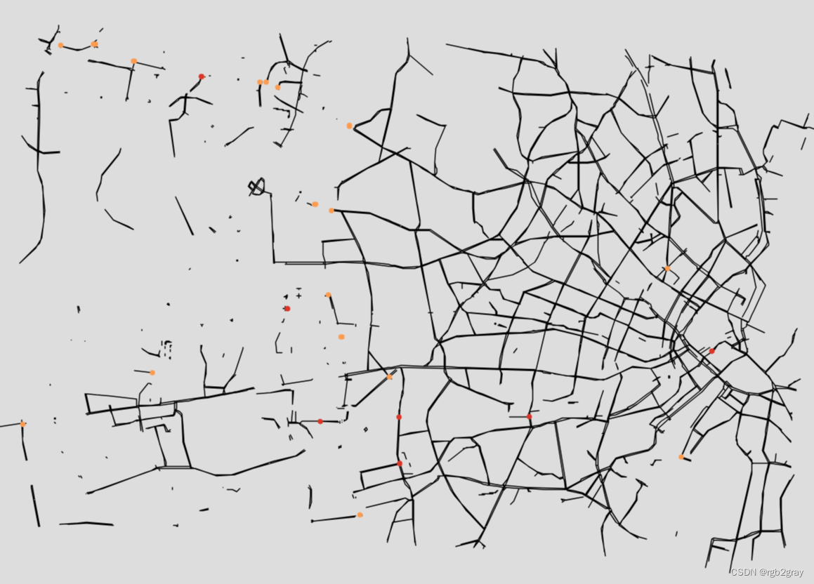
### Overshoots
overshoots = eval_func.find_overshoots(dangling_nodes,ref_edges_simplified,length_tolerance_over,return_overshoot_edges=True,
)print(f"{len(overshoots)} potential overshoots were identified with a length tolerance of {length_tolerance_over} m."
)### Undershoots
undershoot_dict, undershoot_nodes = eval_func.find_undershoots(dangling_nodes,ref_edges_simplified,length_tolerance_under,"edge_id",return_undershoot_nodes=True,
)print(f"{len(undershoot_nodes)} potential undershoots were identified with a length tolerance of {length_tolerance_under} m."
)

21 potential overshoots were identified with a length tolerance of 3 m.
11 potential undershoots were identified with a length tolerance of 3 m.

# Save to csv
overshoots[["edge_id", "length"]].to_csv(ref_results_data_fp + f"overshoot_edges_{length_tolerance_over}.csv", header = ["edge_id", "length (m)"], index = False
)pd.DataFrame(undershoot_nodes["nodeID"].to_list(), columns=["node_id"]).to_csv(ref_results_data_fp + f"undershoot_nodes_{length_tolerance_under}.csv", index=False
)

# Interactive plot over/undershootssimplified_edges_folium = plot_func.make_edgefeaturegroup(gdf=ref_edges_simplified,mycolor=pdict["base"],myweight=pdict["line_base"],nametag="Edges",show_edges=True,
)fg = [simplified_edges_folium]if len(overshoots) > 0 or len(undershoot_nodes) > 0:if len(overshoots) > 0:overshoots_folium = plot_func.make_edgefeaturegroup(gdf=overshoots,mycolor=pdict["ref_emp2"],myweight=pdict["line_emp2"],nametag="Overshoots",show_edges=True,)fg.append(overshoots_folium)if len(undershoot_nodes) > 0:undershoot_nodes_folium = plot_func.make_nodefeaturegroup(gdf=undershoot_nodes,mysize=pdict["mark_emp"],mycolor=pdict["ref_contrast"],nametag="Undershoot nodes",show_nodes=True,)fg.append(undershoot_nodes_folium)m = plot_func.make_foliumplot(feature_groups=fg,layers_dict=folium_layers,center_gdf=ref_nodes_simplified,center_crs=ref_nodes_simplified.crs,)bounds = plot_func.compute_folium_bounds(ref_nodes_simplified)m.fit_bounds(bounds)m.save(ref_results_inter_maps_fp+ f"underovershoots_{length_tolerance_under}_{length_tolerance_over}_reference.html")display(m)if len(undershoot_nodes) == 0:print("There are no undershoots to plot.")
if len(overshoots) == 0:print("There are no overshoots to plot.")

if len(overshoots) > 0 or len(undershoot_nodes) > 0:print("Interactive map saved at " + ref_results_inter_maps_fp.lstrip("../") + f"overundershoots_{length_tolerance_under}_{length_tolerance_over}_reference.html")
else:print("There are no under/overshoots to plot.")

Interactive map saved at results/REFERENCE/cph_geodk/maps_interactive/overundershoots_3_3_reference.html

3.网络组件

4.概括

5.保存结果

后续见链接